Linear Regression using Gradient Descent Part-1

Table of Contents

Introduction

Linear Regression is one of the simplest and most fundamental algorithms in Machine Learning and Statistics. It is used to model the relationship between a dependent variable (target) and one or more independent variables (features). The primary objective is to find the best-fitting line that minimizes the error between the actual and predicted values.

One of the most commonly used optimization techniques in Linear Regression is Gradient Descent. In this blog, we will delve into the mathematical foundation of Gradient Descent and its application in optimizing the parameters of a Linear Regression model.

Understanding Linear Regression

The Hypothesis Function

A Linear Regression model assumes that the relationship between the input variables \( X \) and the output variable \( Y \) is linear. The hypothesis function (prediction function) for simple linear regression (with one feature) is given by:

$$ y(x) = b + x \cdot w $$

where:

• $B =$ Bias term.
• $W =$ Weight term.
• $x =$ Independent variable

For multiple linear regression (with multiple features), the hypothesis function is extended as:

$$ y(x) = b + x_1\cdot w_1 + x_2\cdot w_2 + \; \dots \;+ x_n\cdot w_n $$

Or in vector notation:

$$\hat Y = X \cdot W + B $$

where:

• $X (m \times n)$ is the matrix of input features,
• $W (n \times 1)$ is the vector of parameters (coefficients),
• $B$ is the bias scalar.
• $\hat Y (m \times 1)$ is the predicted output.

The Cost Function

To measure how well our hypothesis function fits the data, we use the Mean Squared Error (MSE), also known as the Cost Function (Loss Function):

$$ L = \frac{1}{2m} \sum_{i=1}^{m} (\hat y(x_i) - y_i)^2 $$

where:

• $m$ is the number of training examples,
• $\hat y(x_i)$ is the predicted value for the $i$-th example,
• $y_i$ is the actual output.

Our goal is to minimize $L$, which means finding the optimal parameters $w \;\; and \;\; b$.

Gradient Descent: Optimization Algorithm

Concept of Gradient Descent

Gradient Descent is an iterative optimization algorithm used to find the minimum of a function. In our case, it helps find the optimal values of $w \;\; and \;\; b$ that minimize the loss function $L$.

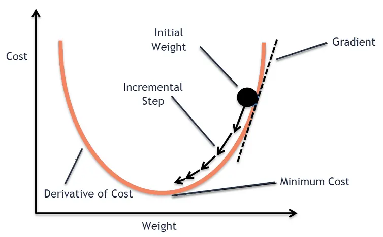
The gradient descent algorithm finds the gradient (or derivative) and then using it tries to move closer to the optimal value.

In the given image above the gradient of the weight at that instance is +ve, so to move towards the optimal value it moves in the opposite direction of the gradient. Hence, the gradients are subtracted.

Similarly, when it is on the left side the gradient is -ve and when moving towards optimal value it increases (as -ve $\times$ -ve = +ve ).

Hence, the algorithm always tries to move along the slope and in a direction opposite to its gradient.

The idea is to start with initial values of $w \;\; and \;\; b$ and update them iteratively using the gradient of the cost function until convergence. The update rule is given by:

$$ w_i = w_i - \alpha \cdot \frac{\partial L}{\partial w_i}$$$$ b = b - \alpha \cdot \frac{\partial L}{\partial b}$$

where:

• $\alpha$ is the learning rate (a small positive number that controls the step size),
• $\frac{\partial \ L}{\partial \ w_i}$ is the gradient (partial derivative of the cost function with respect to $w_j$).

Computing the Gradient

Now we know that $L = \frac{1}{2m} \sum_{i=1}^{m} (\hat y_i - y_i)^2$

$$ \therefore \frac{\partial L}{\partial \hat y} = \frac{1}{2m} \sum_{i=1}^{m} 2 \cdot (\hat y - y) \cdot 1 $$$$ \therefore \frac{\partial L}{\partial \hat y} = \frac{1}{m} \sum_{i=1}^{m} (\hat y - y) $$

We also know that $\hat y = \sum_{i=1}^{m} x_i.w_i + b$

$$ \therefore \frac{\partial \hat y}{\partial w_i} = x_i$$$$ \therefore \frac{\partial \hat y}{\partial b} = 1$$

Hence, the partial derivatives of the cost function are calculated as follows:

$$\frac{\partial L}{\partial w_i} = \frac{\partial L}{\partial \hat y} \cdot \frac{\partial \hat y}{\partial w_i} $$$$\therefore \frac{\partial L}{\partial w_i} = x_i \cdot \frac{1}{m} \sum_{i=1}^{m} (\hat y - y) $$$$\frac{\partial L}{\partial b} = \frac{\partial L}{\partial \hat y} \cdot \frac{\partial \hat y}{\partial b} $$$$\therefore \frac{\partial L}{\partial b} = \frac{1}{m} \sum_{i=1}^{m} (\hat y - y) $$

Thus, the update rule becomes:

$$ w_i = w_i \; - \alpha \cdot \; \frac{\partial L}{\partial w_i} $$$$ b = b \; - \;\alpha \cdot \frac{\partial L}{\partial b}$$

This is applied iteratively until convergence.

Implementing Gradient Descent for Linear Regression

Algorithm Steps

1. Initialize parameters: Set initial values for $w_i=1$ and $b = 0$.
2. Compute the cost function: Calculate the loss $L$ using the given data.
3. Compute the gradient: Determine the partial derivatives.
4. Update parameters: Adjust $w_i \; and \; b$ using the update rule.
5. Repeat until the cost function converges.

Choosing the Learning Rate

The learning rate $\alpha$ is crucial:

• If $\alpha$ is too small, convergence is slow.
• If $\alpha$ is too large, the algorithm may not converge.

Convergence of Gradient Descent

Gradient Descent converges when the change in the cost function is minimal (i.e., when $J(\theta)$ no longer decreases significantly). This can be monitored using:

$$ | Loss(new) - Loss(old) | < \epsilon $$

where $\epsilon$ is a small threshold value.

Conclusion

In this blog, we explored Linear Regression and its optimization using Gradient Descent. We covered the hypothesis function, cost function, gradient descent update rule, and implementation details.

In Part-2, we will implement Linear Regression with Gradient Descent using Python and visualize the learning process. Linear Regression using Gradient Descent Part-2

Stay tuned!

---