Linear Regression using Gradient Descent Part-2
- Raunak Wete
- Machine learning , Python
- March 8, 2025
Table of Contents
Introduction
In this blog we are going to learn on how to implement Linear Regression using Gradient Descent using Python. We will not be directly using ML libraries like scikit-learn but instead do from scratch to increase our understanding. For representing the data we will be using NumPy library as it is efficient and we don’t need to waste our time creating a matrix library.
Before proceeding forward it is necessary to know the basics of Gradient Descent algorithm. Read the previous blog Linear Regression using Gradient Descent Part-1 which explains the theory and the math behind it in detail.
Setting up the Environment
Install python
- For Windows: Download the latest python version 3.13.2
Invoke-WebRequest -Uri "https://www.python.org/ftp/python/3.13.2/python-3.13.2-amd64.exe" `
-OutFile "$env:HOMEPATH\Downloads\python-3.13.2-amd64.exe"; `
Start-Process "$env:HOMEPATH\Downloads\python-3.13.2-amd64.exe"  -Wait; `
Remove-Item "$env:HOMEPATH\Downloads\python-3.13.2-amd64.exe" -Force
- For MacOS:
brew install python
- For Linux(Ubuntu/Debian):
sudo apt install python3 python3-venv
Setup Python
- Create a Python Virtual Environment
mkdir linear_reg
cd linear_reg
python3 -m venv .venv
Note: For Windows users use PowerShell and not cmd for running these commands.
Activate the environment
- For Windows Users:
.\.venv\Scripts\actiavate.ps1- For MacOS / Linux Users:
.venv/bin/activateInstall Necessary Libraries:
pip3 install numpy matplotlib
Python Implementation
Create Dataset
For understanding purpose we will be using a synthetically generated dataset and not an actual dataset. Consider a dataset with 3 features $x_1, x_2, x_3$ and a dependent variable $y$.
Note: We will be using Multiple Linear Regression example but the same will apply for Simple Linear Regression also.
# Import necessary libraries
import numpy as np
import matplotlib.pyplot as plt
# Define x1, x2, x3
x1 = np.random.rand(1000, 1)
x2 = np.random.rand(1000, 1)
x3 = np.random.rand(1000, 1)
X = np.column_stack([x1, x2, x3])

y_true = x1 * 1.5 + x2 * 3.8 + x3 * 4.7 + 8.9 + np.random.randn(1000, 1)
Note: Here $y = 1 \cdot x_1 + 2 \cdot x_2 + 3 \cdot x_3 + \epsilon$ and a random value is added for making the dataset more realistic.
# Split into train and test dataset
X_train, X_test = X[:900], X[900:]
y_train, y_test = y_true[:900], y_true[900:]
Initialize the model parameters
$$y = x_1 \cdot w_1 + x_2 \cdot w_2 + x_3 \cdot w_3 + b $$$$y = X \cdot W + b $$Initialize weights $w_1 = 1$ and bias $b = 0$
# Initialize model parameters
w = np.ones((3, 1))
b = 0

epochs = 1000
lr = 0.01
The value of lr should be carefully adjusted.
- If too low then the model doesn’t converge
- If too high then the model doesn’t fit because of very large changes.
Define Loss
$$ L = \frac{1}{2m} \sum_{i=1}^{m} (\hat y(x_i) - y_i)^2 $$# Define loss
def loss(y_pred, y_true):
return np.mean(np.square(y_pred - y_true)).item()
Training Loop
In the training the gradients are calculated based on the following formulas:
$$\frac{\partial L}{\partial \hat y} = (\hat y - y) $$$$\hat y = X \cdot W + b$$$$\frac{\partial \hat y}{\partial W} = X^T \quad \dots \;\; (\text{Matrix differentiation})$$$$\frac{\partial L}{\partial W} = \frac{\partial L}{\partial \hat y} \cdot \frac{\partial \hat y}{\partial W} $$$$\therefore \frac{\partial L}{\partial W} = X^T \cdot (\hat y - y)$$$$\frac{\partial L}{\partial b} = (\hat y - y) $$And based on these gradients they are updated as follows:
$$ w = w \; - \alpha \cdot \; \frac{\partial L}{\partial w} $$$$ b = b \; - \;\alpha \cdot \frac{\partial L}{\partial b}$$When the loss $\lt 10^{-10} \;\; i.e$ , the loss has converged we stop the training.
# Training Loop
prev_loss = 0
losses = []

for i in range(epochs):
    iter_loss = 0
    for x, y in zip(X_train, y_train):
        x = x.reshape(1, -1)
        y_pred = x @ w + b
        new_loss = loss(y_pred, y)
        iter_loss += new_loss

        dldz = 2 * (y_pred - y)
        dldw = x.T * dldz
        dldb = dldz

        w -= lr * dldw
        b -= lr * dldb

    iter_loss /= len(X_train)
    loss_diff = abs(prev_loss - iter_loss)
    losses.append(iter_loss)

    if loss_diff < 1e-10:
        print(iter_loss)
        print(f"Loss converged in {i + 1} iterations")
        break

    prev_loss = iter_loss
Check the accuracy of our model
We will be using $R^2$ to check our model accuracy. When the model perfectly predicts the outputs then $R^2 = 1$ So, if $R^2$ is closer to 1 then our model is accurate.
$$R^2 = 1 - \frac{\sum_{i=1}^{n} (y_i - \hat y_i)^2}{\sum_{i=1}^{n} (y_i - \bar y)^2}$$where
- $y_i =$ actual value
- $\hat y_i =$ predicted value
- $\bar y =$ mean of $y$
# Define r2_score
def r2_score(y_pred, y_true):
    ssr = np.sum(np.square(y_true - y_pred))
    sse = np.sum(np.square(y_true - np.mean(y_true)))

    return 1 - (ssr/sse)
# Based on the tuned parameters find the loss, r2_score
y_pred = X_test @ w + b

l = loss(y_pred, y_test)
r2 = r2_score(y_pred, y_test)

print(f"Loss = {l}")
print(f"R^2 score = {r2}")
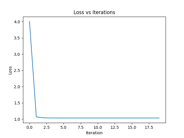
Visualize loss
We will visualize the loss of our model to see if it continuously decreased or not.
# Visualize the loss w.r.t no. of iterations
plt.plot(losses)
plt.title("Loss vs Iterations")
plt.xlabel("Iteration")
plt.ylabel("Loss")
plt.show()
Complete Code
Here is the complete code for linear regression using gradient descent
# Import necessary libraries
import numpy as np
import matplotlib.pyplot as plt

# Define x1, x2, x3
x1 = np.random.rand(1000, 1)
x2 = np.random.rand(1000, 1)
x3 = np.random.rand(1000, 1)
X = np.column_stack([x1, x2, x3])

y_true = x1 * 1.5 + x2 * 3.8 + x3 * 4.7 + 8.9 + np.random.randn(1000, 1)

# Split into train and test dataset
X_train, X_test = X[:900], X[900:]
y_train, y_test = y_true[:900], y_true[900:]

# Initialize model parameters
w = np.ones((3, 1))
b = 0

epochs = 1000
lr = 0.01

# Define Loss function
def loss(y_pred, y_true):
    return np.mean(np.square(y_pred - y_true)).item()

# Training Loop
prev_loss = 0
losses = []

for i in range(epochs):
    iter_loss = 0
    for x, y in zip(X_train, y_train):
        x = x.reshape(1, -1)
        y_pred = x @ w + b
        new_loss = loss(y_pred, y)
        iter_loss += new_loss

        dldz = 2 * (y_pred - y)
        dldw = x.T * dldz
        dldb = dldz

        w -= lr * dldw
        b -= lr * dldb

    iter_loss /= len(X_train)
    loss_diff = abs(prev_loss - iter_loss)
    losses.append(iter_loss)

    if loss_diff < 1e-10:
        print(f"Loss converged in {i + 1} iterations")
        break

    prev_loss = iter_loss

# Define r2_score
def r2_score(y_pred, y_true):
    ssr = np.sum(np.square(y_true - y_pred))
    sse = np.sum(np.square(y_true - np.mean(y_true)))
    return 1 - (ssr / sse)

# Based on the tuned parameters find the loss, r2_score
y_pred = X_test @ w + b
l = loss(y_pred, y_test)
r2 = r2_score(y_pred, y_test)

print(f"Loss = {l}")
print(f"R^2 score = {r2}")

# Print the parameters
print(f"Weight(W) = {w}")
print(f"Bias(b) = {b}")

# Visualize the loss w.r.t no. of iterations
plt.plot(losses)
plt.title("Loss vs Iterations")
plt.xlabel("Iteration")
plt.ylabel("Loss")
plt.show()
Output
# Output
Loss converged in 20 iterations
Loss = 0.9098035015965859
R^2 score = 0.8097464359033948

Weight(W) = [[1.574951 ]
 [3.81217961]
 [4.8721643 ]]
Bias(b) = [[8.80130388]]
As we can see the predicted parameters are close to the actual values
| Parameter | Actual Value | Predicted Value |
|---|---|---|
| $w_1$ | 1.5 | 1.57 |
| $w_2$ | 3.8 | 3.81 |
| $w_3$ | 4.7 | 4.87 |
| $b$ | 8.9 | 8.8 |
Thus, we can use these values to predict values for given features.
Conclusion
In this blog we learned about how to implement the gradient descent algorithm from scratch using python. This is a simple implementation of the algorithm. In actual use batched inputs are used to increase the performance and efficiency.
Libraries like sklearn do a lot of processing and use the most efficient techniques and algorithms to get accurate results quickly.
In the future we will try to implement a Neural Network from scratch based on the above principles.
Stay tuned!.